Tutorials
Introduction to binding sites 
In this tutorial, you will explore the fundamental concepts and computational methods for studying binding sites to enhance your understanding and analysis of molecular interactions.
Table of Contents: 
- Introduction
- Basic concepts
- Types of binding sites
- Computational methods to study binding sites
- DeepChem tools
- How does a binding pocket look like?
- Further Reading
This tutorial is made to run without any GPU support, and can be used in Google colab. If you'd like to open this notebook in colab, you can use the following link.
![]()
Introduction 
Binding sites are specific locations on a molecule where ligands, such as substrates, inhibitors, or other molecules, can attach through various types of molecular interactions.
Binding sites are crucial for the function of many biological molecules. They are typically located on the surface of proteins or within their three-dimensional structure. When a ligand binds to a binding site, it can induce a conformational change in the protein, which can either activate or inhibit the protein's function. This binding process is essential for numerous biological processes, including enzyme catalysis, signal transduction, and molecular recognition.
For example, in enzymes, the binding site where the substrate binds is often referred to as the active site. In receptors, the binding site for signaling molecules (such as hormones or neurotransmitters) is critical for transmitting signals inside the cell.
Understanding binding sites is particularly relevant for the development of new drugs, as it can lead to the development of more effective and selective drugs from multiple angles:
- Target identification: Identifying binding sites on target proteins allows researchers to design molecules that can specifically interact with these sites, leading to the development of drugs that can modulate the protein's activity.
- Drug design: Knowledge of the structure and properties of binding sites enables the design of drugs with high specificity and affinity, reducing off-target effects and increasing efficacy.
- Optimization: Detailed understanding of binding interactions helps improving the binding characteristics of drug candidates, such as increasing binding affinity and selectivity.
Additionally, knowledge of the structure and properties of binding sites enables the design of drugs with high specificity and affinity, reducing off-target effects and increasing efficacy.

Myoglobin (blue) with its ligand heme (orange) bound. Based on PDB: 1MBO.
Basic concepts 
Here we cover some basic notions to understand the science of binding site identification.
Molecular Interactions 
The specific interactions that occur at the binding site can be of various types, including (non-exhaustive list):
-
Hydrogen Bonding: Weak electrostatic interactions between hydrogen atoms bonded to highly electronegative atoms (like oxygen, nitrogen, or fluorine) and other electronegative atoms or functional groups. Hydrogen bonding is important for stabilizing protein-ligand complexes and can be enhanced by halogen bonding.
-
Halogen Bonding: A type of intermolecular interaction where a halogen atom (like iodine or fluorine) acts as an acceptor, forming a bond with a hydrogen atom or a multiple bond. Halogen bonding can significantly enhance the affinity of ligands for binding sites.
-
Orthogonal Multipolar Interactions: Interactions between backbone carbonyls, amide-containing side chains, guanidinium groups, and sulphur atoms, which can also enhance binding affinity.
-
Van der Waals Forces: Weak, non-specific interactions arising from induced electrical interactions between closely approaching atoms or molecules. They usually provide additional stabilization and contribute to the overall binding affinity, especially in close-contact regions.
-
Metal coordination: Interactions between metal ions (e.g., zinc, magnesium) and ligands that have lone pairs of electrons (e.g., histidine, cysteine, water). These interactions are typically coordinate covalent bonds, where both electrons in the bond come from the ligand, and are crucial in metalloenzymes and metalloproteins, where metal ions often play a key role in catalytic activity and structural stability.
-
Polar Interactions: Interactions between polar functional groups, such as hydrogen bond donors (e.g., backbone NH, polarized Cα–H, polar side chains, and protein-bound water) and acceptors (e.g., backbone carbonyls, amide-containing side chains, and guanidinium groups).
-
Hydrophobic Interactions: Non-polar interactions between lipophilic side chains, which can contribute to the binding affinity of ligands.
-
Pi Interactions: Interactions between aromatic rings (Pi-Pi), and aromatic rings with other types of molecules (Halogen-Pi, Cation-Pi,...). They occur in binding sites with aromatic residues such as phenylalanine, tyrosine, and tryptophan, and stabilize the binding complex through stacking interactions.
 Valiulin, Roman A. "Non-Covalent Molecular Interactions". Cheminfographic, 13 Apr. 2020,
https://cheminfographic.wordpress.com/2020/04/13/non-covalent-molecular-interactions
Valiulin, Roman A. "Non-Covalent Molecular Interactions". Cheminfographic, 13 Apr. 2020,
https://cheminfographic.wordpress.com/2020/04/13/non-covalent-molecular-interactions
Ligands 
Ligands are molecules that bind to specific sites on proteins or other molecules, facilitating various biological processes.
Ligands can be classified into different types based on their function:
- Substrates: Molecules that bind to an enzyme's active site and undergo a chemical reaction.
- Inhibitors: Molecules that bind to an enzyme or receptor and block its activity.
- Activators: Molecules that bind to an enzyme or receptor and increase its activity.
- Cofactors: Non-protein molecules (metal ions, vitamins, or other small molecules) that bind to enzymes to modify their activity. They can act as activators or inhibitors depending on the specific enzyme and the binding site.
- Signaling Lipids: Lipid-based molecules that act as signaling molecules, such as steroid hormones.
- Neurotransmitters: Chemical messengers that transmit signals between neurons and their target cells.

Protein Ligand Docking. Adobe Stock #216974924.
The binding of ligands to their target sites is influenced by various physicochemical properties:
- Size and Shape: Ligands must be the appropriate size and shape to fit into the binding site.
- Charge: Electrostatic interactions, such as ionic bonds, can contribute to ligand binding.
- Hydrophobicity: Hydrophobic interactions between non-polar regions of the ligand and the binding site can stabilize the complex.
- Hydrogen Bonding: Hydrogen bonds between the ligand and the binding site can also play a crucial role in binding affinity.
The specific interactions between a ligand and its binding site, as well as the physicochemical properties of the ligand, are essential for understanding and predicting ligand-receptor binding events
Binding Affinity and Specificity 
Binding affinity is the strength of the binding interaction between a biomolecule (e.g., a protein or DNA) and its ligand or binding partner (e.g., a drug or inhibitor). It is typically measured and reported by the equilibrium dissociation constant ($K_d$), which is used to evaluate and rank the strengths of bimolecular interactions. The smaller the $K_d$ value, the greater the binding affinity of the ligand for its target. Conversely, the larger the $K_d$ value, the more weakly the target molecule and ligand are attracted to and bind to one another.
Binding affinity is influenced by non-covalent intermolecular interactions, such as hydrogen bonding, electrostatic interactions, hydrophobic interactions, and van der Waals forces between the two molecules. The presence of other molecules can also affect the binding affinity between a ligand and its target.
Binding specificity refers to the selectivity of a ligand for binding to a particular site or target. Highly specific ligands will bind tightly and selectively to their intended target, while less specific ligands may bind to multiple targets with varying affinities. It is determined by the complementarity between the ligand and the binding site, including factors such as size, shape, charge, and hydrophobicity (see section above on ligands). Specific interactions, like hydrogen bonding and ionic interactions, contribute to the selectivity of the binding.
Binding specificity is crucial in various biological processes, such as enzymatic reactions or drug-target interactions, as it allows for specific and regulated interactions, which is essential for the proper functioning of biological systems.
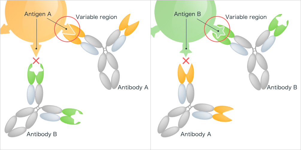
Antigen-antibody interactions are particularly highly specific binding sites (often also characterized by high affinity). The specificity of these interactions is fundamental to ensure precise immune recognition and response. Kyowa Kirin. "Specificity of Antibodies".
In summary, binding affinity measures the strength of the interaction between a ligand and its target, while binding specificity determines the selectivity of the ligand for a particular binding site or target.
Thermodynamics of Binding 
The thermodynamics of binding involves the interplay of enthalpy ( $𝐻$), entropy ($S$), and Gibbs free energy ($G$) to describe the binding of ligands to binding sites. These thermodynamic parameters are crucial in understanding the binding process and the forces involved.
- Enthalpy ($H$) is a measure of the total energy change during a process. In the context of binding, enthalpy represents the energy change associated with the formation of the ligand-binding site complex. A negative enthalpy change indicates that the binding process is exothermic, meaning that heat is released during binding. Conversely, a positive enthalpy change indicates an endothermic process, where heat is absorbed during binding.
- Entropy ($S$) measures the disorder or randomness of a system. In binding, entropy represents the change in disorder associated with the formation of the ligand-binding site complex. A negative entropy change indicates a decrease in disorder, which is often associated with the formation of a more ordered complex. Conversely, a positive entropy change indicates an increase in disorder, which can be seen in the disruption of the binding site or the ligand.
- Gibbs free energy ($G$) is a measure of the energy change during a process that takes into account both enthalpy and entropy. It is defined as $G = H - TS$, where $T$ is the temperature in Kelvin. Gibbs free energy represents the energy available for work during a process. In binding, a negative Gibbs free energy change indicates that the binding process is spontaneous and favorable, while a positive Gibbs free energy change indicates that the process is non-spontaneous and less favorable.

Calculated variation of the Gibbs free energy (G), entropy (S), enthalpy (H), and heat capacity (Cp) of a given reaction plotted as a function of temperature (T). The solid curves correspond to a pressure of 1 bar; The dashed curve shows variation in ∆G at 8 GPa. Ghiorso, Mark S., Yang, Hexiong and Hazen, Robert M. "Thermodynamics of cation ordering in karrooite (MgTi2O5)" American Mineralogist, vol. 84, no. 9, 1999, pp. 1370-1374. https://doi.org/10.2138/am-1999-0914
- Binding isotherms are models that describe the relationship between the concentration of ligand and the occupancy of binding sites. These isotherms are crucial in understanding the binding process and the forces involved. One example is the Langmuir isotherm, which assumes that the binding site is homogeneous and the ligand binds to the site with a single binding constant.
- Cooperative binding occurs when the binding of one ligand molecule affects the binding of subsequent ligand molecules. This can lead to non-linear binding isotherms, where the binding of ligands is enhanced or inhibited by the presence of other ligands. Cooperative binding is often seen in systems where multiple binding sites are involved or where the binding site is heterogeneous.
Kinetics of Binding 
The kinetics of binding involves the study of the rates at which ligands bind to and dissociate from binding sites.
- Rate constants for association and dissociation are essential in describing the kinetics of binding. They represent the rate at which the ligand binds or dissociates to the site, respectively.
- Kinetic models are used to describe the binding process. One commonly used kinetic model to describe enzyme kinetics is the Michaelis-Menten model, which assumes that the enzyme has a single binding site and that the binding of the substrate is reversible. There are other kinetic models, including the Langmuir adsorption model.

Binding curves for three ligands following the Hill-Langmuir model, each with a $K_d$ (equilibrium dissociation constant) of 10 µM for its target protein. The blue ligand shows negative cooperativity of binding, meaning that binding of the first ligand reduces the binding affinity of the remaining site(s) for binding of a second ligand. The red ligand shows positive cooperativity of binding, meaning that binding of the first ligand increases the binding affinity of the remaining site(s) for binding of a second ligand. "Hill-Langmuir equation". Open Educational Alberta. https://openeducationalberta.ca/abcofpkpd/chapter/hill-langmuir/ .
Types of binding sites 
Binding sites can be classified based on various criteria depending on the context. This is a non-exhaustive list of binding sites categories based on the type of molecule they bind to:
-
Protein Binding Sites: These are regions on a protein where other molecules can bind. They can be further divided into:
- Active Sites: Regions where enzymes bind substrates and catalyze chemical reactions. Example: The active site of the enzyme hexokinase binds to glucose and ATP, catalyzing the phosphorylation of glucose.
- Allosteric Sites: Regions where ligands bind and alter the protein's activity without being part of the active site. Example: The binding of 2,3-bisphosphoglycerate (2,3-BPG) to hemoglobin enhances the ability of hemoglobin to release oxygen where it is most needed.
- Regulatory Sites: Regions where ligands bind and regulate protein activity or localization. Example: Binding of a regulatory protein to a specific site on a receptor can modulate the receptor's activity.
-
Nucleic Acid Binding Sites: These are regions on DNA or RNA where other molecules can bind. They can be further divided into:
- Transcription Factor Binding Sites: Regions where transcription factors bind to regulate gene expression. Example: The TATA box is a DNA sequence that transcription factors bind to initiate transcription.
- Restriction Sites: Regions where restriction enzymes bind to cleave DNA. Example: The EcoRI restriction enzyme recognizes and cuts the DNA sequence GAATTC.
- Recombination Sites: Regions where site-specific recombinases bind to facilitate genetic recombination. Example: The loxP sites are recognized by the Cre recombinase enzyme to mediate recombination.
-
Small Molecule Binding Sites: These are regions on proteins or nucleic acids where small molecules like drugs or substrates bind. They can be further divided into:
- Compound Binding Sites: Regions typically located at the active site of the enzyme where the substrate binds and undergoes a chemical reaction, usually reversible. Example: The binding site for the drug aspirin on the enzyme cyclooxygenase (COX) inhibits its activity.
- Cofactor Binding Sites: Regions where cofactors can bind, sometimes permanently and covalently attached to the protein, and can be located at various sites. Example: The binding site for the heme cofactor in hemoglobin, which is essential for oxygen transport.
- Ion and Water Binding Sites: These are regions on proteins or nucleic acids where ions or water molecules bind. The calcium-binding sites in calmodulin, which are crucial for its role in signal transduction.
Computational methods to study binding sites 
Multiple computational methods have been developed in the last decades to study and identify binding sites, offering insights that complement experimental approaches. These methods enable the prediction of binding affinities, the identification of potential drug candidates, and the understanding of the dynamic nature of binding interactions. Here are some key computational approaches used to study binding sites:
| Method | Description | Applications | Tools | Output |
|---|---|---|---|---|
| Molecular Docking | Predicts the preferred orientation of a ligand when bound to a protein or nucleic acid binding site. | Used extensively in drug discovery to screen large libraries of compounds and identify potential drug candidates. | AutoDock, Glide, DOCK | Binding poses, binding affinities, interaction maps |
| Molecular Dynamics (MD) Simulations | Provides a dynamic view of the binding process by simulating the physical movements of atoms and molecules over time. | Used to study the stability of ligand binding, conformational changes, and the effect of mutations on binding affinity. | GROMACS, AMBER, CHARMM | Trajectories of atomic positions, binding free energies, insights into the flexibility and dynamics of binding sites |
| Quantum Mechanics/Molecular Mechanics (QM/MM) Methods | Combines quantum mechanical calculations for the active site with molecular mechanical calculations for the rest of the system. | Used to study reaction mechanisms, electronic properties, and the role of metal ions in binding sites. | Gaussian, ORCA, Q-Chem | Detailed electronic structure information, reaction pathways, energy profiles |
| Homology Modeling | Predicts the 3D structure of a protein based on the known structure of a homologous protein. | Useful for studying binding sites in proteins for which no experimental structure is available. | MODELLER, SWISS-MODEL, Phyre2 | Predicted 3D structures that can be used for docking and MD simulations |
| Virtual Screening | Computationally screens large libraries of compounds to identify potential ligands that bind to a target binding site. | Widely used in drug discovery to prioritize compounds for experimental testing. | Schrodinger's Glide, AutoDock Vina, GOLD | Ranked lists of compounds with predicted binding affinities and poses |
| Machine Learning and AI | Uses machine learning and AI techniques to predict binding affinities, identify binding sites, and generate new ligand structures. | Enhancing the accuracy of docking predictions, predicting drug-target interactions, and designing novel compounds. | DeepChem, TensorFlow, PyTorch, protein language models (ESM2) | Predictive models, binding affinity predictions, novel ligand designs |
| Protein-Ligand Interaction Fingerprints (PLIF) | Computational representations of the interactions between a protein and a ligand. | Used to compare binding modes, identify key interactions, and cluster similar binding sites. | MOE, Schrödinger's Maestro | Interaction maps, similarity scores |
Recently, large language models, particularly protein language models (PLMs), have emerged as powerful tools for predicting protein properties. These models typically use a transformer-based architecture to process protein sequences, learning relationships between amino acids and protein properties. PLMs can then be fine-tuned for specific tasks, such as binding site prediction, reducing the need for large, specific training datasets and offering high scalability.
DeepChem tools for studying binding sites 
DeepChem in particular has a few tools and capabilities for identifying binding pockets on proteins:
- BindingPocketFinder : This is an abstract superclass in DeepChem that provides a template for child classes to algorithmically locate potential binding pockets on proteins. The idea is to help identify regions of the protein that may be good interaction sites for ligands or other molecules.
- ConvexHullPocketFinder : This is a specific implementation of the BindingPocketFinder class that uses the convex hull of the protein structure to find potential binding pockets. It takes in a protein structure and returns a list of binding pockets represented as CoordinateBoxes.
- Pose generators : Pose generation is the task of finding a “pose”, that is a geometric configuration of a small molecule interacting with a protein. A key step in computing the binding free energy of two complexes is to find low energy “poses”, that is energetically favorable conformations of molecules with respect to each other. This can be useful for identifying favorable binding modes and orientations (low energy poses) of ligands within a protein's binding site. Current implementations allow for Autodock Vina and GNINA.
- Docking : There is a generic docking implementation that depends on provide pose generation and pose scoring utilities to perform docking.
There is a tutorial on using machine learning and molecular docking methods to predict the binding energy of a protein-ligand complex, and another tutorial on using atomic convolutions in particular to model such interactions.
How does a binding site look like? 
Let's visualize a binding pocket in greater detail. For this purpose, we need to download the structure of a protein that contains a binding site. As an illustrative example, we show here a well-known protein-ligand pair: the binding of the drug Imatinib (Gleevec) to the Abl kinase domain of the BCR-Abl fusion protein, which is commonly associated with chronic myeloid leukemia (CML). The PDB ID for this complex is '1IEP'.
# setup
!pip install py3Dmol biopython requests
import requests
import py3Dmol
from Bio.PDB import PDBParser, NeighborSearch
from io import StringIO
Requirement already satisfied: py3Dmol in /usr/local/lib/python3.10/dist-packages (2.1.0)
Requirement already satisfied: biopython in /usr/local/lib/python3.10/dist-packages (1.83)
Requirement already satisfied: requests in /usr/local/lib/python3.10/dist-packages (2.31.0)
Requirement already satisfied: numpy in /usr/local/lib/python3.10/dist-packages (from biopython) (1.25.2)
Requirement already satisfied: charset-normalizer<4,>=2 in /usr/local/lib/python3.10/dist-packages (from requests) (3.3.2)
Requirement already satisfied: idna<4,>=2.5 in /usr/local/lib/python3.10/dist-packages (from requests) (3.7)
Requirement already satisfied: urllib3<3,>=1.21.1 in /usr/local/lib/python3.10/dist-packages (from requests) (2.0.7)
Requirement already satisfied: certifi>=2017.4.17 in /usr/local/lib/python3.10/dist-packages (from requests) (2024.6.2)
# Download the protein-ligand complex (PDB file)
pdb_id = "1IEP"
url = f"https://files.rcsb.org/download/{pdb_id}.pdb"
response = requests.get(url)
pdb_content = response.text
Let's see what's inside the pdb file:
# Parse the PDB content to identify chains and ligands
chains = {}
for line in pdb_content.splitlines():
    if line.startswith("ATOM") or line.startswith("HETATM"):
        chain_id = line[21]
        resn = line[17:20].strip()
        if chain_id not in chains:
            chains[chain_id] = {'residues': set(), 'ligands': set()}
        chains[chain_id]['residues'].add(resn)
        if line.startswith("HETATM"):
            chains[chain_id]['ligands'].add(resn)
chains_info = chains
print("Chains and Ligands Information:")
for chain_id, info in chains_info.items():
    print(f"Chain {chain_id}:")
    print(f"  Residues: {sorted(info['residues'])}")
    print(f"  Ligands: {sorted(info['ligands'])}")
Chains and Ligands Information:
Chain A:
  Residues: ['ALA', 'ARG', 'ASN', 'ASP', 'CL', 'CYS', 'GLN', 'GLU', 'GLY', 'HIS', 'HOH', 'ILE', 'LEU', 'LYS', 'MET', 'PHE', 'PRO', 'SER', 'STI', 'THR', 'TRP', 'TYR', 'VAL']
  Ligands: ['CL', 'HOH', 'STI']
Chain B:
  Residues: ['ALA', 'ARG', 'ASN', 'ASP', 'CL', 'CYS', 'GLN', 'GLU', 'GLY', 'HIS', 'HOH', 'ILE', 'LEU', 'LYS', 'MET', 'PHE', 'PRO', 'SER', 'STI', 'THR', 'TRP', 'TYR', 'VAL']
  Ligands: ['CL', 'HOH', 'STI']
We have a homodimer of two identical chains and several ligands: CL, HOH, and STI. CL and HOH are common solvents and ions binding to the protein structure, while STI is the ligand of interest (Imatinib).
For visualization, let's extract the information of chain A and its ligands:
chain_id = "A"
chain_lines = []
for line in pdb_content.splitlines():
    if line.startswith("HETATM") or line.startswith("ATOM"):
        if line[21] == chain_id:
            chain_lines.append(line)
    elif line.startswith("TER"):
        if chain_lines and chain_lines[-1][21] == chain_id:
            chain_lines.append(line)
chain_A = "\n".join(chain_lines)
view = py3Dmol.view()

# Add the extracted chain model
view.addModel(chain_A, "pdb")

# Set the styles
view.setStyle({'cartoon': {'color': 'darkgreen'}})
for ligand in chains_info[chain_id]['ligands']:
    view.addStyle({'chain': 'A', 'resn': ligand}, {'stick': {'colorscheme': 'yellowCarbon'}})
view.zoomTo()

view.show()
3Dmol.js failed to load for some reason. Please check your browser console for error messages.
Now let's highlight the binding pocket in the protein ribbon. For this purpose we need to parse the PDB content again to identify residues belonging to chain A and STI ligand:
parser = PDBParser()
structure = parser.get_structure('protein', StringIO(pdb_content))

# Extract residues of chain A and the ligand STI
str_chain_A = structure[0][chain_id]
ligand = None
ligand_resname = "STI"
for residue in structure.get_residues():
    if residue.id[0] != ' ' and residue.resname == ligand_resname:
        ligand = residue
        break
if ligand is None:
    raise ValueError("Ligand STi not found in the PDB content")

chain_A_atoms = [atom for atom in str_chain_A.get_atoms()]
ligand_atoms = [atom for atom in ligand.get_atoms()]
/usr/local/lib/python3.10/dist-packages/Bio/PDB/StructureBuilder.py:89: PDBConstructionWarning: WARNING: Chain A is discontinuous at line 5038.
  warnings.warn(
/usr/local/lib/python3.10/dist-packages/Bio/PDB/StructureBuilder.py:89: PDBConstructionWarning: WARNING: Chain B is discontinuous at line 5079.
  warnings.warn(
/usr/local/lib/python3.10/dist-packages/Bio/PDB/StructureBuilder.py:89: PDBConstructionWarning: WARNING: Chain A is discontinuous at line 5118.
  warnings.warn(
/usr/local/lib/python3.10/dist-packages/Bio/PDB/StructureBuilder.py:89: PDBConstructionWarning: WARNING: Chain B is discontinuous at line 5217.
  warnings.warn(
Now we can find the residues in chain A within a certain distance from the ligand. Here we set this distance to 5Å.
binding_residues = set()
distance_threshold = 5.0
ns = NeighborSearch(chain_A_atoms)

for ligand_atom in ligand_atoms:
    close_atoms = ns.search(ligand_atom.coord, distance_threshold)
    for atom in close_atoms:
        binding_residues.add(atom.get_parent().id[1])
And let's see the visualization, now with the binding pocket:
# Create a py3Dmol view
view = py3Dmol.view()

# Add the chain model
view.addModel(chain_A, "pdb")

# Set the style for the protein
view.setStyle({'cartoon': {'color': 'darkgreen'}})

# Color the binding pocket residues
for resi in binding_residues:
    view.addStyle({'chain': chain_id, 'resi': str(resi)}, {'cartoon': {'colorscheme': 'greenCarbon'}})

# Color the ligand
view.addStyle({'chain': chain_id, 'resn': ligand_resname}, {'stick': {'colorscheme': 'yellowCarbon'}})

# Zoom to the view
view.zoomTo()

# Show the view
view.show()
3Dmol.js failed to load for some reason. Please check your browser console for error messages.
Further Reading 
For further reading on computational methods for binding sites and protein language models here are a couple of great resources:
Congratulations! Time to join the Community! 
Congratulations on completing this tutorial notebook! If you enjoyed working through the tutorial, and want to continue working with DeepChem, we encourage you to finish the rest of the tutorials in this series. You can also help the DeepChem community in the following ways:
Citing this tutorial 
If you found this tutorial useful please consider citing it using the provided BibTeX.
@manual{Bioinformatics,
 title={Introduction to Binding Sites},
 organization={DeepChem},
 author={Gómez de Lope, Elisa},
 howpublished = {\url{https://github.com/deepchem/deepchem/blob/master/examples/tutorials/Introduction_to_Binding_Sites.ipynb}},
 year={2024},
}